
Every month (around the 15th) the national public safety system (SNSP) releases information regarding the number of crimes commited in Mexico, this information comes from the local (state) district attorney's office who compile information about the number of crimes commited for something like 10 or so different fellonies and then submit it to the SNSP who publishes the data at the state and national level.
Due to the constant release of data, this particular database proves particularly useful for government reporting about the state of public safety in the country for a particular month. Nevertheless consecutive month comparison may not be possible because not all months are created equal (I'll explain further in the next paragraphs). So Alejandro Hope and me at IMCO decided it could be good idea to create a database that we could compare easily with any other month of the database (which runs from 1997 to the present). We chose to focus our efforts on the homicide (intentional) time series. We chose this particular series for a couple of very simple reasons. Homicide is probably the crime with the lowest under reportment rate (which should in theory also render it the most consistent in the database), and it's certainly the most serious crime, which should then help us assess the state of public safety better than the other available crimes.
First of all, why should we expect marked monthly differences in crime rates? Well the first reason is that different months have a different number of days. So, even at the same rate of homicides per day, consecutive months can vary around 3% without real changes in the underlying situation. This is even more serious in the case of February which, at current numbers, can have about 150 more homicides than January or March at the same average number of homicides per day. But then, why not use average homicides per day as our benchmark? Well it might also be that the number of days per month doesn't tell the whole story.
The most interesting theory of why different months can have different crimes rates is the so called summer effect which associates higher crime rates to the summer months. It's two main arguments are the following. Firstly vacation periods of school age children and adolecents, therefore they have more idle time in which occupy themselves and might lead to criminal behavior, aditionally they spend more time outside increasing some criminal oportunities. Aditionally weather might also play a part here, people are more likely to be out in the warmer times of the year and even temperature itself might turn people to become more criminally inclined. These theories have often been studied and most of the evidence leans towards it beign correct even if the full causality is not very clear.
We knew of a series of techniques that are used to remove these ciclical factors from time series, this is a procedure known as seasonal adjustment. But before actually getting to the adjustment phase we had to inspect the series to look for marked differences between months, so we built a seasonal factors graph by period. This graph helps us see how the number of homicides for a particular month varies from the yearly mean and also how this variation changes over time. Meaning that for example, on average, May is has about 10% more homicides than the yearly average and February around 10% less.
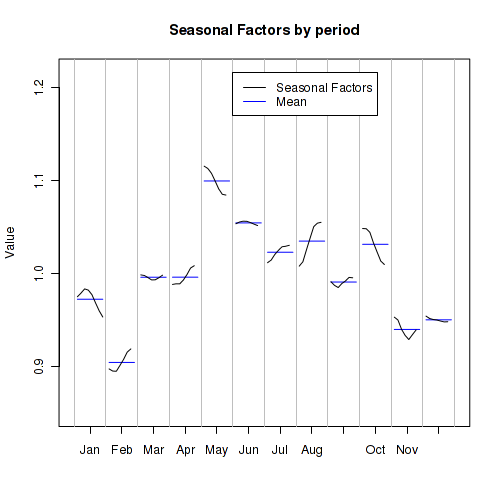
This hints at the Summer Effect theory. As we can see in the previous graph, the months between May and August all show substancially higher numbers than average figures. On the contrary the colder months (November, December, January and February) clearly lower numbers than the rest of the year. This, and several statistical tests for seasonality, convinced us that the intentional homicide time series showed seasonality. So our next step was to adjust the series to remove those cyclical effects.
Presently the two most commonly used seasonal adjustment methods are X-13 Arima, developed by the U.S. Census Bureau, and TRAMO/SEATS, which was developed by Spain's central bank. These two are basically a series of econometric procedures that are applied to the original series that output three new series. A trend series, a seasonal component series and an irregular component series (there is also a cyclical component for longer runs). Basically any time series can be disagregated into these components and the sum of the three will yield the original series. In it's most basic form the seasonal component only includes that part of the series that comes from the seasonal effect. The trend component describes the basic inertia of the series and resembles somehow a moving average in that it greatly smooths the series behavior. Finally the irregular component includes those parts of the series that could be considered as shocks, for example the San Fernando Massacre in April 2011 that included nearly 200 homicides in a single event, which can greatly impact the series but don't necessarly alter the underlying trend. So if we remove that seasonal component from the original series we would come up with a seasonaly adjusted series and the observations in this new series can be compared with any other month of the series, a bit like inflation adjustment.
These two methods, X-13-Arima and TRAMO/SEATS, are quite similar and also produce quite similar results. In the past my method of choice had been TRAMO/SEATS (via Gretl) but that often required me to use multiple software usually by the way of cumbersome shell scripts. So when I heard about a new R package (my weapon of choice) that linked X-13 and R I decided to switch to that. While the installation and linking can be a bit of hassle the package runs smoothly and having everything in the same workspace speeds up the analysis. So after quite a while picking the most appropiate model specification (complete code in my GitHub) we end up with the seasonally adjusted time series.
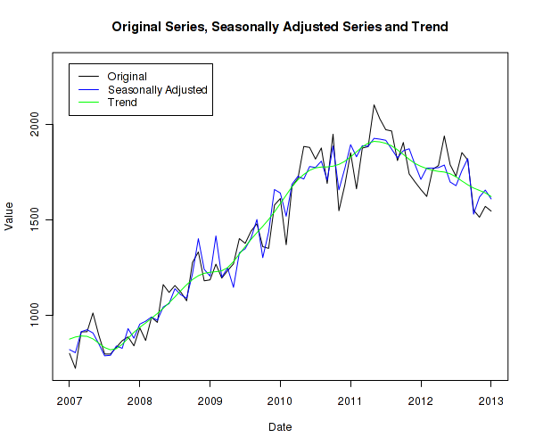
The previous graph shows the combination of the 3 series; original, seasonally adjusted and trend series. It's easy to see that perhaps the main advantage of such graph is that we can see interesting months easily. For example 2011, the most dire period in our public safety crisis. The year started out with what in the original series would have been seen as a decreasing number of homicides but as the summer came about those figures spiraled upwards of 2,000 homicides per month, when we include the seasonally adjusted and trend series we can see that the reduction in February and March was mostly due to seasonal effects and the huge bump in April, May and June was also mostly normal, meaning that while the number of homicides per month was on the rise, the real slope wasn't as steep as it seemed.
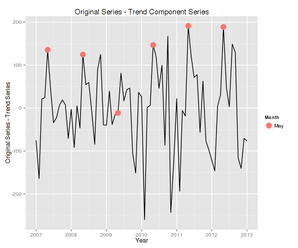
The thing that I find the most puzzling is May. While it might not be the most violent month of the year for the whole series, mostly due to the ever increasing homicide numbers between 2007 and 2011, it certainly is the most violent for those periods where the trend is relatively stable. Actually if we remove the trend component (basically keeping the cyclical, seasonal and irregular components) out of the series, we find that for the years 2007-2012 May is the month with the highest number of homicides for 4 out of the 6 years (and a very close second for 2010). What this means is that if we exclude the rate of change of the series then May is certainly the most violent month of the year for almost the whole series. The question here is why is May so violent?
We've had multiple conversations here in the office about May. While the summer effect might be some sort of explanation, if this were true we would still expect the following months to be more violent than May. The two main ideas behind the summer effect should be better explained by months such as July and August, mainly higher temperatures and more people on vacation and out and about. Particularly because while most Secundarias and Preparatorias (junior and senior high school) don't have school starting at the end of May and because temperatues are higher on average on June and July than in May. So any alternative theories would be greatly appreciated.
So let's get to some final conclusions. The main reason behind exercise was to provide a time series of intentional homicide in Mexico that could be comparable with any other month of the series so we could provide some information about the evolution and current situation of that indicator. Using this database we have so far created three monthly reports about the evolution of violence in Mexico for the months of March, April and May (see them here; March , April and May. Apart from that data you can also see some other cool things in there such as maps of homicide numbers per state and some pretty neat scenario calculators). The main conclusions in those reports are that, while violence still seems to be decreasing, the trend is not as downwards steep as we would like and as the official reports show. The main reason is because traditionally the first months of the year have a lower number of homicides than the latter months, for this reason the raw data shows much lower figures than the adjusted data and in the end the yearly totals should, in theory, even out after the end of the summer months.
For the first 5 months of the year the raw change with respect to the same period of last year is about -13% but when we compare it with the seasonaly adjusted data of the last 5 months of 2012 this change ends up being about -7%, considerable lower than what the unadjusted data would show, this would put us on par to have between 19 and 20 thousand prelimary investigations for intentional homicide by the end of the year, slightly less than the 2012 numbers. Nevertheless there is still hope for the future, May 2013 proved to be quite a good month for us, while the raw variations versus April 2013 was only 1.8% the seasonally adjusted data shows a -6.3% improvement for the month, hopefully this should turn into a trend.
PS: You can download all the data such as the adjusted time series at the IMCO reports.